A few weeks back, I posted some images that I put together by combining old maps with recent aerial photographs. Since then, I’ve discovered how to import those same maps into Google Earth. This is really exciting, because it allows you to explore these maps in an interactive way. Instead of being stuck with an orthogonal ‘straight down’ view, you can move around and view things from any angle you choose. A gallery of examples is below. In these images are three different historical maps:

• ‘Plan of the limits of the town of Brisbane’ (1843). You can see the original in the Queensland Historical Atlas.
• ‘Plan of Portions 203 to 257 in the Environs of Brisbane, Parish of Enoggera, County of Stanley, New South Wales’ (1859). This is available at the Queensland State Archives (Item ID620656) and the State Library (Record 727379).
• ‘Plan of Brisbane Water Works’ (1864). This map shows the pipeline route between Enoggera Reservoir and Brisbane City, and is available from the Brisbane City Council Archives.

Boundary Creek as depicted on in 1864. In the foreground is the Coronation Drive Office Park, and behind it is Suncorp Stadium.

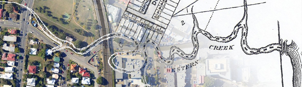
The course of Western Creek through Norman Buchan Park, Fernberg and Rosalie, as depicted in 1864.

Looking down the Milton Reach, with Langsville Creek in the foreground and Western Creek in the middle, as depicted in 1859.

Looking over Western Creek (as depicted in 1859) towards Suncorp Stadium and the city. In the immediate foreground is Dunmore Park.

The reservoir and creek that once flowed through the CDB, as depicted in 1843. Also visible is the Old Windmill on Spring Hill.

The creek that once flowed from Spring Hill, down through Roma Street (where it was dammed), and through King George Square and the CBD, as depicted in 1843.

Your turn!

The best bit about bringing these maps into Google Earth is that they can be shared, since Google Earth is freely available. To explore the maps shown in the images above, simply download the following files and load them into Google Earth. (Usually you can just double-click the files once you have downloaded them. Otherwise, you can drag them straight from your file browser into Google Earth, or open the from within Google Earth by selecting ‘File’ and then ‘Open’.) Of course, you will need to download and install Google Earth if you don’t have it already.

• 1843-plan-of-brisbane-png.kmz (367 KB)
• 1859-parish-of-enoggera-png.kmz (1 MB) (Note that this map is only properly aligned on the Milton side of the river — sorry!)
• 1864-plan-of-waterworks-png.kmz (345 KB)

These files will produce results much like those in the images above, but are not quite the same. They do not align quite as well to the modern terrain, and they lack the ‘shadow’ effect that is applied in the above examples. However, they are smaller, crisper and more reliable. If you want to use the same files as I used for the images, here they are:

• 1843-plan-of-brisbane.kmz (1.5MB)
• 1859-parish-of-enoggera.kmz (4.3MB) (Note that this map is only properly aligned on the Milton side of the river — sorry!)
• 1864-plan-of-waterworks.kmz (1.5MB)

However, before you use this second set of files, please note the following:

• These files take a long time to load in Google Earth. When you open them, you will need to wait for a while (as long as 30 seconds) before Google Earth will respond and display the map.
• On some occasions, Google Earth may crash when opening these files. This seems to happen mostly when there is already another one of these files displaying. So before you open one, ensure that you have unchecked (in the left-hand panel) any others that you have already loaded.
• Treat these files as experimental, and nothing more. They are ‘proof-of-concept’, but could do with a lot more refinement, which I may or may not ever get around to doing.

If you have any trouble getting these to work, or want to provide some feedback, feel free to leave a comment at the bottom of this page. Have fun!

How they were made

For anyone who is interested, here is a brief run-down of how I prepared these maps for importing into Google Earth:

1. I loaded the original map in Photoshop, and converted it into a monochrome (black and white) image using a ‘Threshold’ layer. This turns the background of the map (and any lightly coloured features) solid white, and makes the dark features of the map pure black. I then inverted the resulting image, making the background black and the features white.
2. I used the eraser tool to manually clean up the ‘noise’ (white specks) that resulted from the first step. (I was not especially thorough in some maps, so you will still see some rogue specks here and there.)
3. I added the resulting image as a raster layer in ArcMap (a professional mapping program) and ‘geo-rectified’ it by matching its features to those on a layer that was already geographically aligned (an aerial photo, for example). This can be tricky, especially if there are few roads or other common features on the original map (as was the case with the 1843 plan of Brisbane). By telling ArcMap to make all of the black parts of the map transparent, I was left with just the white features.
4. I converted this raster layer to a polygon layer, and then converted that to a kmz file, using a native tool in ArcMap. I would have done this without first creating a polygon layer, but for some reason the conversion tool would not work straight from the raster. At first this seemed like a pointless step, but it does allow you to tailor the appearance of the kmz by first adjusting the line style. I’ve experimented with various line styles, and so far yellow (with a fine black border) seems to be the colour that is easiest to see over the Google Earth aerial imagery.

The steps above describe the files second set of downloads. The files in the first set were created a bit differently. Instead of converting the raster to a polygon layer, I edited it in photoshop and saved it as a PNG (portable network graphic) file with the background already transparent (the PNG format allows transparent pixels, while JPEG does not). I then added the PNG file as an overlay image in Google Earth, and stretched it until it aligned with the streets and other features. This alignment process is not as sophisticated as that allowed in ArcMap, so the alignment is not quite as good. Finally, I saved it as a KMZ file from within Google Earth.

There are probably still other ways of doing this, so if you have any alternate methods to share, I’d love to hear them!